


2. For a system with input plane at the origin x = 0 and lenses spaced out from the origin and then from each other by 200, 100, 50, and 75mm, of focal lengths 300, -200, 80, and -150 respectively, same questions. CB's program for parts 1 and 2 is 13 lines, using the functions described below.
3. Make a plot of one or both these systems showing the path followed by the ray you used to find the focal length. Hint: I think the following one is right for 2:
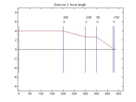
These plots, and graphics in general, are nice for intuition and debugging and actually necessary in tutorial and expository scientific writing. Matlab makes them easy, so why not practice? The most important information is the trace of the ray, the rest is "just labels", but mysterious graphics can turn off your reader. Maybe you could cobble together a plot interactively, maybe mark up a simple matlab in a graphics editor like photoshop....but if you automate the production of a complex plot you are amply repaid when you want to do several, or something similar.
4. A) You know enough to write the ray transfer matrix for an optical
flat, so please do so. Let's say it's in air, with two parallel surfaces normal to the optic
axis Lmm apart, and its glass's index of refraction is
4. B) Sketch the ray-trace diagram of a couple of rays at different angles passing through the flat. Describe in words its effect on a ray.
5. (Extra Credit). Why invest all this work and not play around with the result a little? The three-lens system in the second plot has lenses spaced out by 300, 100, and 50 of focal lengths 200, -50, and 50. According to Prof. T, Brown's notes [1], it is a simplified the form of a telephoto lens, whose job is to let you vary the linear magnification without changing the image plane so the image stays in focus while zooming. Complex optical systems are not easy to design, and involve tradeoffs between image quality, efficient and controlled light flux, and appropriate flexibility for the application.
See if you can turn the system into a telephoto lens. I assumed, remembering real cameras we see, that pushing the lefthand lens backwards toward the origin, thus making the system longer, would increase linear magnification. But I also figured that maybe we could compensate that by moving the 2nd lens.
I used a system with lenses spaced by 300mm, 100mm, 50mm from the origin, of focal lengths 100mm, -50mm, and 50mm. My findings are pretty unexciting: it works, but there's not much magnification. There's a slightly nonlinear dependency relationship on lens1 motion and both compensation and magnification. At this point it's clearly time to read the textbook or take the optical instrumentation course.
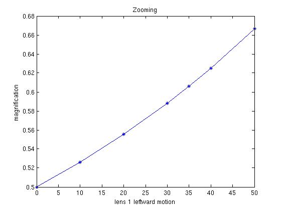
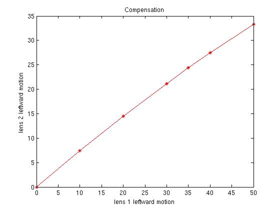
So have a shot yourself. Start with some similar system; numbers don't have to be same as mine. Maybe investigate how the first lens's focal length affects magnification, maybe change f.l. of lens 2, maybe try deviations of lens 1 to the right as well as left. Make some plots to summarize what you find. As an engineer, how would you mechanically design a zoom lens so that twisting one "zoom" control ring moves two (sets of) lenses at different rates?
Graphics are really useful for debugging and for demonstration. A plot can be really simple: one horizontal line for the central (X) axis, one vertical line for the input plane, output plane (if any), and each lens, and the ray trace. All the labels can be moved in the caption. The value added by my display function probably isn't worth the effort for this exercise.
I figure it makes sense to have a function (cbray below) that takes in a description of the optical system and an initial ray. For ray plotting, I knew I wanted to produce the table of the ray's (x, y) at the origin, the image plane, and at all the lenses. I discovered I could also produce the final ray's description (for finding the focal length or axial image point (image plane), and I returned the final 2x2 system matrix (strictly for curiosity, never used).
System representation: since I need to constuct the system matrix by multiplying two different (translation, thin-lens) types of matrices together, my description has top row with a code for each element type (0 translation, 1 thin lens). Both elements only need a single parameter (distance, focal length), so that information is in the second row below the appropriate code. A system description could look like this:
[0   1   0   1   0  1 ;
200 200 100 -50 50 50];
(Some of the ray-transfer matrices have more parameters, up to four for the thick lens, so we'd need more rows to include them in our system.) A ray is a 2-row column vector with y and angle values).
cbray initializes a ray vector V to the input ray and initializes system, translate, and thin-lens matrices to the identity, and constructs a matrix for the (x,y) pairs that's the right size. The rest of it is just one for-loop with a switch statement inside that loops through the system description columns and modifies the translate or thin-lens matrix as appropriate, and does the element-matrix*V multiplication to get the new ray and the element-matrix*system-matix multiplication to get the new system matrix. If the operation is a translation, we also fill in the next row of the (x,y) matrix we want to return using the x from the system description input and the y from the current ray we just updated. 25 lines total.
To make one of those plots, the ray is just a plot of the (x,y) matrix's column 1 versus column 2. I used line to construct the vertical lines at every x-value in the (x,y) matrix.
My display routine (see above disclaimer and probably ignore this!) showrays(xys, labels) thus takes the (x,y) matrix for the ray but also a 2-column description of labels on the vertical lines that is directly calculatable from the system description matrix if you like: you want a line at the origin, at every lens, and after any final translation. So I probably didn't need this extra bit of representation. Shoot. My label array looks like this:
[0,0; % for source plane or origin
1, 200; % for lenses
1, -50;
1, 50];
0, 0]  % for image plane
each row has two numbers: (type, focallength). Types: 0 for no label (used for origin (input plane) and output-planes), a 1 for lens. Focallength: unused for type 0, converted for lenses. Also its sign determines whether to use the X or V label. I convert the focal length to a string for text. So part of that process looks like this:
if (labels(i,1) == 1 && labels(i,2) > 0)
     text(rayxys(i,1),height+1, 'X');
     text(rayxys(i,1), height + 2, num2str(labels(i,2)));
end
Total of 18 lines.
Thus my main.m script has a lot of this sort of thing:
sysdesc = [0   1   0   1 0 1 ;    %three lenses
          200 200 100 -50 50 50];

rayyang = [4;0];  % ray  (y, angle), parallel to axis to get focal length

[xys1, fray,sysmat] = cbray(sysdesc, rayyang)  %trace the ray

labels = [0,0; 1, 200; 1, -50; 1, 50]; & info to help create plot
figure;
showrays(xys1, labels);  % pretty picture
title('Example 1');
foclength = -fray (1) / fray(2)  %  compute focal length from final ray.
5. Telephoto Experiment: The basic operation is to get the image distance and magnification of a system. function [fm] = focmag(sysdesc) does that, just as you did for problems 1 and 2 of this assignment. In fact if I'd written focmag first, my main script for getting those distances and magnifications would have been simpler. It returns the 2-vector [image-distance magnification]. 12 lines.
The main function runfocmag(sysdesc, delta1, delta2) takes the usual system description and the distance to move lenses 1 and 2. It prints the results of running focmag(sysdesc) and similarly after first moving lens 1 and then moving lens 2. For every delta1, we want the delta2 that will put the image distance back to its original value. I was going to automate the search for the right amount, but the relation between the two turned out to be almost linear and it was easier to search interactively: send in different delta2s chosen by estimation and refinement. I got image-distance agreement down to .01 mm or less for each different value of delta1. 7 lines.
Make some plots something like those below (same situation seen from two points of view). Here, the green circle is ray origin, rays are red, intersection points are blue. Try enough different plane coefficients, bundles, and points of view to make sure both you and your reader believe that everything works as desired. For instance, a small number of rays lets you look along them to see if they are hitting the plane where you want (see below). Viewing the intersection points from the right angle should project them all up into a line (ditto).
All this assignment boils down to is: put the single-ray and plane intersection solution from the reading inside a for-loop with a plot.
Note: it's neat (and good professional practice)
to make direction vectors (for us, the ray's
αs)
always be unit vectors,
and ditto for the (A,B,C) coefficients of the plane equation. That
means that all distances (e.g. the distance of a point from
the plane) are in the same units (then d,
the stretch factor of the
ray, also is the distance of the ray's origin to
the intersection.) But we don't use these distances nor compare them,
so we can just pick any three numbers for our α's and
coefficients.
If we want to normalize each to a unit vector before use, fine; if
not,
fine too; our answers won't vary in this exercise. Below, I don't.
We can still visualize what the plane-through-origin coefficients
That freedom means we can easily make a bundle of rays. Pick a "principal α" that is the average direction of the ray bundle. Then just add a random 0-mean 3-vector to it, and repeat for as many rays as you need. For this work I assume a uniform random distribution, so use rand().
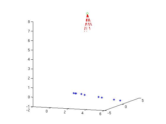
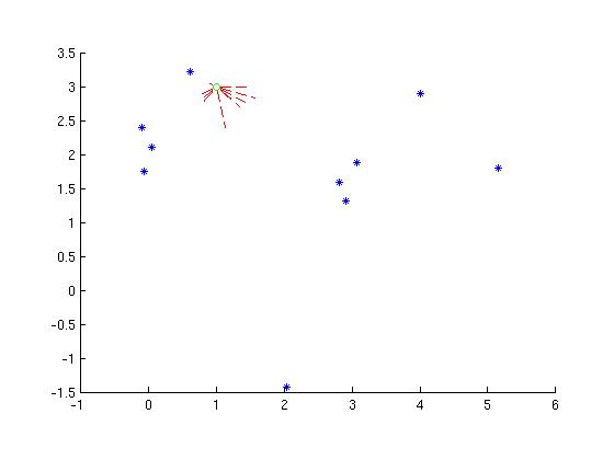
Here's a possible main script for the above approach: (5 lines)
X0 = [1; 3; 8]; %ray origin
a = [.1;-.2; -1];  %looking not quite straight down, on average
N=11;  % how many rays
P = [0.1, 0.2, 1]; % unnormalized plane eqn
% initialization done... now go for it!
x2cbcast(X0,a, N, P); %casts, displays both...
Here are my functions (partial code, code, English...):
This main function does
everything given intialization: (7 lines including 2 ends)
function inter = x2cbcast(X0, a, N, P)
% returns intersection array for N rays of average
% direction a; X0, a are COLUMN vectors.
% P alane coeff. 3-vec (A,B,C).

% here have doubly nested for loop calling function cbcast
% to cast N*N rays, return
% the "inter" array of intersections.

set maximum perturbation magnitude;
for N rays
 create perturbed a,  called perturb
 call solve_one for that ray to get intersection point
 x2cbdisp(X0,perturb,inter);  % plot it all...
 end %end for
end  % end function
Display:
The following plotting function works OK for me. Use or modify as
you like, but your style and
representations may differ, so at least make sure you understand
the use of plot3.
function x2cbdisp(X0, a,inter)
mag = 1.5;
a = mag*a;   % to make rays display at a reasonable length
xend = X0+a;  % end of displayed ray

plot3([X0(1),xend(1)],[X0(2),xend(2)],[X0(3),xend(3)],'r--');
   % plot the red rays
plot3([inter(1)],[inter(2)],[inter(3)],'b*');
   % plot their intersection with the plane
plot3([X0(1)], [X0(2)], [X0(3)],'go');
   % plot X0 % (N times! pretty ugly...)
hold on;   % another ray may be coming up
daspect([1,1,1]);  % kill autoscaling
view(30,30);  % force 3-D plot somehow (!?)
end
Casting A Ray: (7 lines)
function inter = solve_one(x0, alpha, P)
This function is called N times in x2cbcast to create the 3-D
intersection points of the rays from origin x0 in direction α
and the plane with coefficients given by P.
It implements the mathematics in the reading.
You'll remember that we compute (as the third row of the Almost Final Answer), d, the stretch factor that puts the ray on the plane. Adding that times α to X0 should give the intersection point, a 3-d point on the ray such that its dot product with the plane coefficients is 0. Likewise you can check here that inter dotted with P is also zero. Nice to know before you trust the answer.
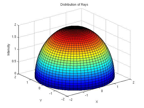
This just needs the quadratic equation and the same ray-casting idea you've used. Here is a good start; I find that our (X0, α) approach gives neater results than his two-point aproach to defining a line, though. The answer is clearly radially symmetric. A symbolic solution would be nice, but plot (use surf) would be lovely. Either or both is fine.
B) What's the distribution over the (tilted) plane Ax+By+Cz = 0? Clearly the symmetrical function of A) gets skewed as it's projected on the tilted plane. Easiest computational approach here, I bet, is to start with the set-up used for part A) -- α points down the z axis. Then for every ray used to create the plot in A), intersect it with the tilted plane instead, and plot the brightness of the ray (from A)) as a function of the (x,y) of that intersection.
If the ray origin is infinitely far away, the rays are parallel. Also cartesian coordinates work fine. About 5 lines of Matlab (plus surf-labeling ones) gives
Extra:If you had extra fun, the derivation and a plot or two would be really cool.